The previous article covered finding TALE loci in one genome at a time. A real study usually has several genomes, and the interesting question becomes “which TALEs, across strains, are versions of the same thing”: alleles of one locus, related by descent. This article covers that comparison: tales_compare_distal() to quantify how alike every pair of arrays and domains is, and tales_group_hclust()/tales_group_kmedoids() to turn that into discrete groups.
1 Discovering TALEs across several genomes
This is a fresh discovery run, independent of the previous article, over three related genomes: MAI1, BAI3, and the best-corrected version of BAI3-1-1 from the correction section of the mining article.
Why only three genomes
tantale ships a fourth sample genome, PXO86, a distantly related Asian outgroup strain. It is left out here deliberately: its TALE repertoire barely overlaps the African strains’ at all, so including it turns a clean set of one-locus-per-strain groups into a mix of real cross-strain groups and PXO86-only paralog clusters, which illustrate a different question from the one this article is asking.
Discovery runs independently per genome, so the article writes it as one function applied to each genome name in turn:
Code
out <- fs::dir_create(file.path(tempdir(), "tale_classification"))
genome_files <- c(
  MAI1       = tantale_genome("MAI1"),
  BAI3       = tantale_genome("BAI3"),
  `BAI3-1-1` = tantale_genome("BAI3-1-1")
)
Code
discover_strain <- function(strain) {
  strain_dir <- file.path(out, strain)
  invisible(tell_tales(subject_file = genome_files[strain], output_dir = strain_dir,
                       cterm_min_score = 300,
                       correct_array = TRUE, max_comparisons = 50))
  tales_from_telltales(strain_dir) |>
    mutate(array_id = paste0(strain, "_", array_id), strain = strain)
}
correct_array = TRUE, with the default max_comparisons = 50, is the route the mining article found clean for BAI3-1-1. Run on MAI1 and BAI3 too, it costs a little extra time; neither needed correcting.
Code
if (fs::file_exists(discovery_cache)) {
  all_tales <- readRDS(discovery_cache)
} else {
  all_tales <- lapply(names(genome_files), discover_strain) |>
    suppressWarnings() |>
    bind_rows()
}
The code prefixes array_id with the strain before combining the three objects, since tell_tales() numbers regions independently within each genome: without the prefix, MAI1’s ROI_00001 and BAI3’s ROI_00001 would collide.
Code
all_tales <- tales(all_tales, sanitize = TRUE)
saveRDS(all_tales, discovery_cache)
n_distinct(all_tales$array_id)
#> [1] 26
Nine arrays each come from MAI1 and BAI3, and eight from BAI3-1-1. plot() with facet_by = "strain" draws one panel per strain:
Code
plot(all_tales, facet_by = "strain")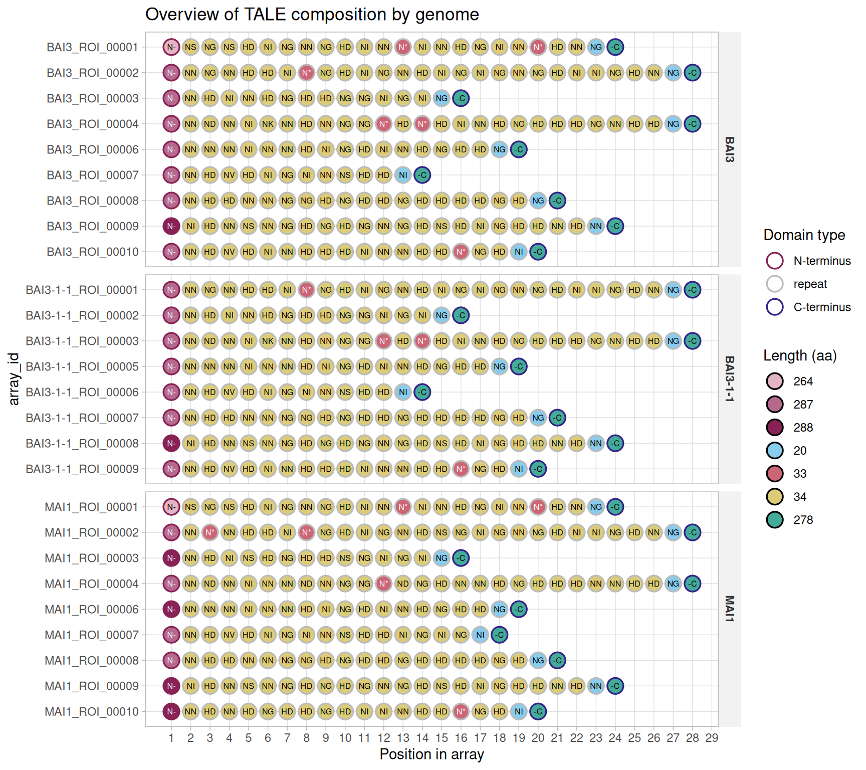
2 Quantifying relatedness: tales_compare_distal()
tales_compare_distal() is tantale’s R implementation of the DisTAL comparison used by the original QueTAL suite: it assigns every distinct domain sequence a dom_code (see the tales class article for what that means), computes pairwise distances between distinct domains, and from those, distances between whole arrays.
Code
if (fs::file_exists(compare_cache)) {
  cmp <- readRDS(compare_cache)
} else {
  cmp <- tales_compare_distal(all_tales, aln_method = "DECIPHER", ncores = 4)
  saveRDS(cmp, compare_cache)
}
names(cmp)
#> [1] "tales"            "domain_distances" "tale_distances"
Code
cmp$tale_distances
#> # A tibble: 676 × 5
#>    id1                id2                dissim arlem_score max_length
#>    <chr>              <chr>               <dbl>       <dbl>      <int>
#>  1 BAI3-1-1_ROI_00001 BAI3-1-1_ROI_00001 0                0         28
#>  2 BAI3-1-1_ROI_00002 BAI3-1-1_ROI_00001 5.64           158         28
#>  3 BAI3-1-1_ROI_00003 BAI3-1-1_ROI_00001 4.89           137         28
#>  4 BAI3-1-1_ROI_00005 BAI3-1-1_ROI_00001 5.14           144         28
#>  5 BAI3-1-1_ROI_00006 BAI3-1-1_ROI_00001 6.07           170         28
#>  6 BAI3-1-1_ROI_00007 BAI3-1-1_ROI_00001 5.32           149         28
#>  7 BAI3-1-1_ROI_00008 BAI3-1-1_ROI_00001 5.04           141         28
#>  8 BAI3-1-1_ROI_00009 BAI3-1-1_ROI_00001 5.46           153         28
#>  9 BAI3_ROI_00001     BAI3-1-1_ROI_00001 4.5            126         28
#> 10 BAI3_ROI_00002     BAI3-1-1_ROI_00001 0.0714           2         28
#> # ℹ 666 more rows
2.1 Does the choice of backend matter?
Comparing domain sequences, the step just run, is the expensive part, and three backends can do it: "DECIPHER" (the default, used above), "Biostrings", and "mmseq2". All three score pairwise protein alignments between domains, so the choice should depend on what is installed and how large the dataset is, and should not change the answer. A small independent fixture, on which all three run quickly, checks that:
Code
small <- tales_from_telltales(system.file("extdata", "tellTaleExampleOutput",
                                          package = "tantale"))
Code
cmp_decipher   <- tales_compare_distal(small, aln_method = "DECIPHER")
cmp_biostrings <- tales_compare_distal(small, aln_method = "Biostrings")
#>
  |
  |                                                                      |   0%
  |
  |=                                                                     |   2%
  |
  |===                                                                   |   4%
  |
  |====                                                                  |   6%
  |
  |======                                                                |   9%
  |
  |=======                                                               |  11%
  |
  |=========                                                             |  13%
  |
  |==========                                                            |  15%
  |
  |============                                                          |  17%
  |
  |=============                                                         |  19%
  |
  |===============                                                       |  21%
  |
  |================                                                      |  23%
  |
  |==================                                                    |  26%
  |
  |===================                                                   |  28%
  |
  |=====================                                                 |  30%
  |
  |======================                                                |  32%
  |
  |========================                                              |  34%
  |
  |=========================                                             |  36%
  |
  |===========================                                           |  38%
  |
  |============================                                          |  40%
  |
  |==============================                                        |  43%
  |
  |===============================                                       |  45%
  |
  |=================================                                     |  47%
  |
  |==================================                                    |  49%
  |
  |====================================                                  |  51%
  |
  |=====================================                                 |  53%
  |
  |=======================================                               |  55%
  |
  |========================================                              |  57%
  |
  |==========================================                            |  60%
  |
  |===========================================                           |  62%
  |
  |=============================================                         |  64%
  |
  |==============================================                        |  66%
  |
  |================================================                      |  68%
  |
  |=================================================                     |  70%
  |
  |===================================================                   |  72%
  |
  |====================================================                  |  74%
  |
  |======================================================                |  77%
  |
  |=======================================================               |  79%
  |
  |=========================================================             |  81%
  |
  |==========================================================            |  83%
  |
  |============================================================          |  85%
  |
  |=============================================================         |  87%
  |
  |===============================================================       |  89%
  |
  |================================================================      |  91%
  |
  |==================================================================    |  94%
  |
  |===================================================================   |  96%
  |
  |===================================================================== |  98%
  |
  |======================================================================| 100%
cmp_mmseq2     <- tales_compare_distal(small, aln_method = "mmseq2")
as.matrix() on a tale_distances object always returns ids sorted the same way, so the three backends’ outputs line up without any further work:
Code
backend_dists <- tibble::tibble(
  DECIPHER   = as.vector(as.matrix(cmp_decipher$tale_distances)),
  Biostrings = as.vector(as.matrix(cmp_biostrings$tale_distances)),
  mmseq2     = as.vector(as.matrix(cmp_mmseq2$tale_distances))
)
cor(backend_dists)
#>             DECIPHER Biostrings    mmseq2
#> DECIPHER   1.0000000  0.9986910 0.9994917
#> Biostrings 0.9986910  1.0000000 0.9988094
#> mmseq2     0.9994917  0.9988094 1.0000000
All three agree closely on this fixture (correlations of 0.998 and above), so the default gives up nothing in accuracy here, at least on data this size.
3 Allocating arrays to groups: tales_group_hclust() and tales_group_kmedoids()
Two clustering methods turn tale_distances into discrete groups. Both take the tales object the distances were computed from, which lets each check that the two actually correspond, and both return it with the result attached as a group column. Each carries its own method-specific arguments (k_range/seed for k-medoids, plot_tree for hclust).
tales_group_kmedoids() fits cluster::pam() for each candidate group count in k_range and plots the average silhouette value of each fit. k = "auto" picks the elbow of that curve, the point after which adding groups stops paying off, a feature tantale adds on top of what DisTAL itself offers:
Code
grouped <- tales_group_kmedoids(cmp$tales, cmp$tale_distances,
                                k_range = 2:20, k = "auto")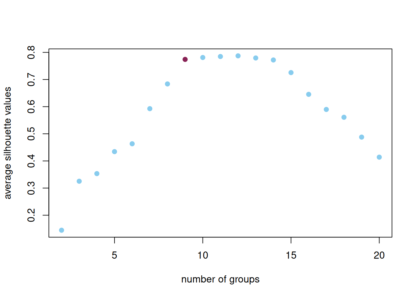
#> The number of groups is automatically decided based on the silhouette value: 9
saveRDS(grouped, group_cache)The automatic pick, in wine on the silhouette plot, is 9 groups. The curve is nearly flat just past it, so a few more groups would fit about as well; the elbow takes the smallest of those. The result is clean: 8 of 9 groups have exactly three members, one from each strain, the one-locus-per-strain pattern this comparison is meant to recover. The remaining group has only a MAI1 and a BAI3 member, matching BAI3-1-1’s one fewer array.
tales_group_hclust() instead cuts a dendrogram at a height chosen to yield exactly k groups, and with plot_tree = TRUE draws it. The tree is a useful check on whether the chosen k looks reasonable:
Code
invisible(tales_group_hclust(cmp$tales, cmp$tale_distances,
                             k = n_distinct(grouped$group),
                             plot_tree = TRUE))
#> ! # Invaild edge matrix for <phylo>. A <tbl_df> is returned.
#> ! # Invaild edge matrix for <phylo>. A <tbl_df> is returned.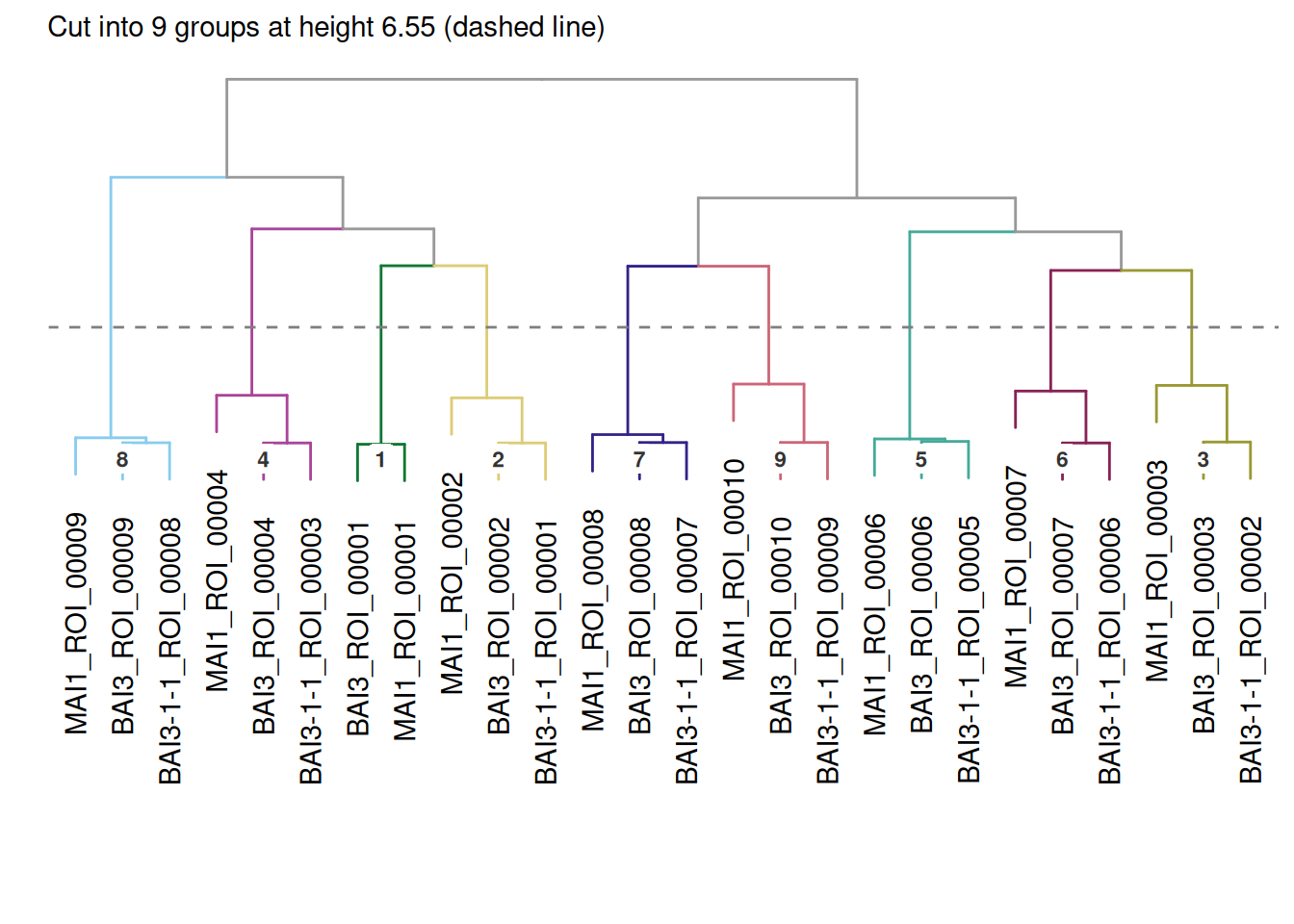
4 An overview across strains: talomes_heatmap()
With arrays assigned to groups, one natural summary is which RVD sequence variant each strain carries in each group. A strain’s talome, by analogy to its genome, is the whole complement of TALEs it carries. grouped already holds a group and a strain for each array, and talomes_heatmap() computes the RVD sequences itself.
Code
talomes_heatmap(grouped, group_col = "group", strain_col = "strain")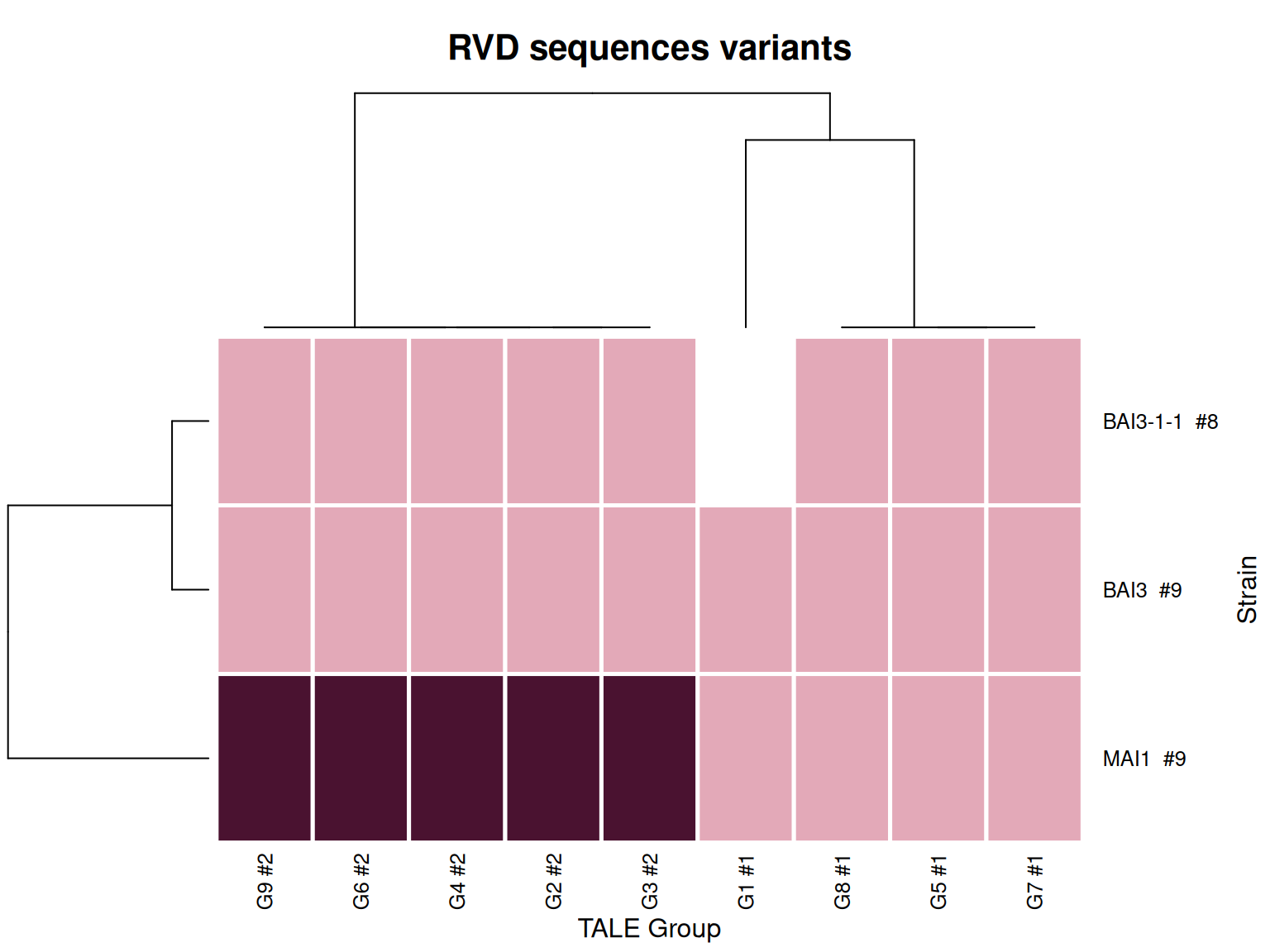
Each cell in Figure 3 is one strain’s RVD sequence variant in one group, coloured by the variant’s rank within that group (the palest is the most common); the # after each group name counts its distinct variants. A white cell means the strain has no member in that group, and a cell split into several colours would mean a strain carries more than one variant in the group. Here, BAI3 and BAI3-1-1 carry the same variant in every group they share. MAI1 carries that same variant in four groups and a different one in the other five.
5 A different lens: comparing predicted binding specificity
Everything above compares TALEs by their sequence, domain by domain, via DisTAL. A TALE’s RVDs also predict, base by base, the DNA sequence it binds, and two arrays can be compared on that prediction directly instead: tales_to_universalmotif() converts each array’s RVD sequence into a position weight matrix (PWM) of DNA-binding preferences, using the same per-RVD specificity weights tales_predict_targets() relies on (rvd_dna_specificity), and tales_compare_functal() scores every pair of PWMs with universalmotif::compare_motifs():
Code
picked_group <- grouped |> filter(group == 6)
functal_dissim <- tales_compare_functal(picked_group)
functal_dissim
#> # A tibble: 9 × 3
#>   id1                id2                dissim
#>   <chr>              <chr>               <dbl>
#> 1 BAI3-1-1_ROI_00006 BAI3-1-1_ROI_00006   0
#> 2 BAI3_ROI_00007     BAI3-1-1_ROI_00006   0
#> 3 MAI1_ROI_00007     BAI3-1-1_ROI_00006   0.25
#> 4 BAI3-1-1_ROI_00006 BAI3_ROI_00007       0
#> 5 BAI3_ROI_00007     BAI3_ROI_00007       0
#> 6 MAI1_ROI_00007     BAI3_ROI_00007       0.25
#> 7 BAI3-1-1_ROI_00006 MAI1_ROI_00007       0.25
#> 8 BAI3_ROI_00007     MAI1_ROI_00007       0.25
#> 9 MAI1_ROI_00007     MAI1_ROI_00007       0
BAI3 and BAI3-1-1, which share the same genomic background, predict the identical binding specificity for this array. MAI1’s version carries the same twelve RVDs followed by four more, and its dissimilarity of 0.25 reflects those four extra positions. This result comes from DNA-binding prediction alone, independently of the DisTAL comparison above, and agrees with it.
Once arrays are a list of real universalmotif motifs, that package’s own plotting functions apply directly. motif_tree() draws the same kind of relatedness tree as tales_group_hclust(), built from binding-specificity distance instead of protein-domain distance:
Code
motifs <- tales_to_universalmotif(picked_group)
universalmotif::motif_tree(motifs, layout = "rectangular", linecol = "none",
                           labels = "name", legend = FALSE) +
  ggplot2::scale_x_continuous(expand = ggplot2::expansion(mult = c(0.02, 0.6)))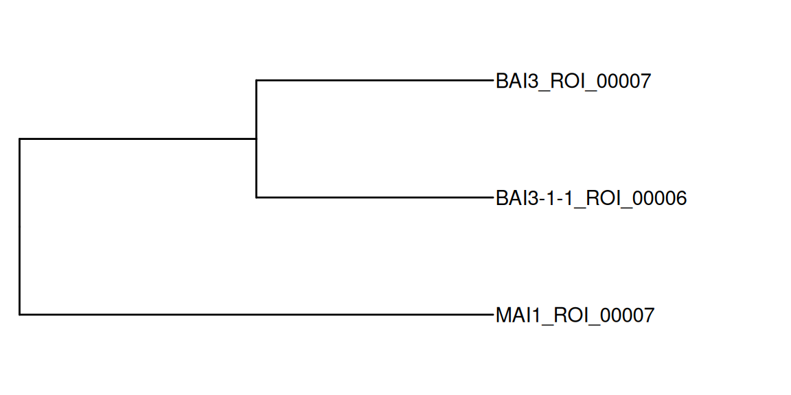
view_motifs() renders the PWMs themselves as sequence logos, showing the specificity model behind the distances. MAI1’s four extra positions are visible at the end:
Code
universalmotif::view_motifs(motifs)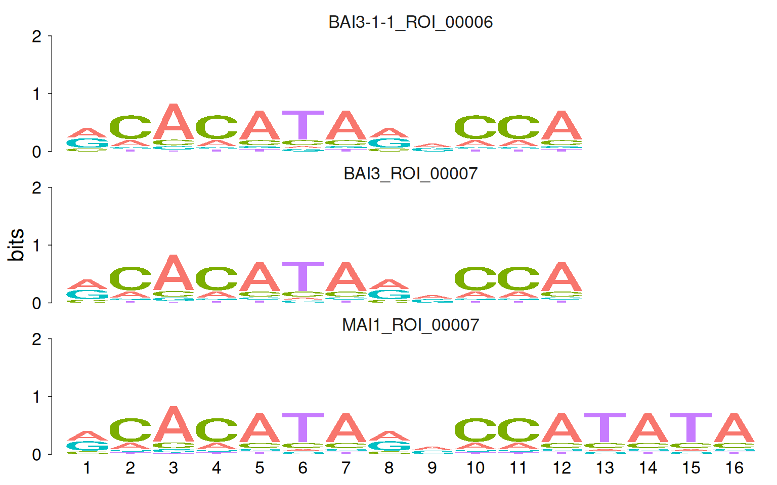
tales_to_universalmotif()’s output is a plain list of universalmotif objects, so the rest of that package’s toolkit is reachable the same way: universalmotif::scan_sequences() can search a promoter sequence for predicted binding sites directly from one of these PWMs, an alternative angle on what tales_predict_targets() does in the target-prediction article; universalmotif::merge_motifs() can build one consensus binding-site model for a whole group, complementing what tales_consensus() already does at the RVD/dom_code layer; and universalmotif::average_ic() is worth checking before comparing motifs at all, since a PWM built from an array with many unresolved RVDs carries little real information and can distort a comparison (0.59 bits here, above the 0.25-bit minimum compare_motifs() applies by default). Statistical significance testing for these comparisons (compare_motifs()’s compare.to/max.p arguments) is deliberately not shown here: universalmotif’s default null distributions are calibrated on real transcription-factor motifs, and applying them to TALE-derived PWMs would give uncalibrated p-values. A TALE-specific calibration is separate work.
6 Next
Grouping tells you which arrays are related. Seeing exactly how (which repeats match, which are inserted or deleted relative to one another) needs an alignment, which is the subject of the next article.