The previous articles found TALE arrays, grouped them, and aligned related ones. This last article asks the question a TALE’s RVD sequence exists to answer: what DNA sequence does it bind? Each RVD contacts one base of the target through a well-characterised, largely one-to-one code (NI prefers A, HD prefers C, NG prefers T, NN prefers G or A, and so on), so a whole RVD sequence predicts an EBE (Effector Binding Element) as a short DNA motif with one position per RVD.
tantale wraps two independent predictors that use this code differently enough to be worth contrasting: TALVEZ, a position-weight-matrix scan, and PrediTALE, which also models where a real EBE tends to sit relative to a transcription start site. Both are wrapped as talvez() and preditale(), which take the same inputs and return the same core columns in the same order (tale_id, rvds, subj_seq_id, start, end, strand, ebe_seq, score), so their predictions can be compared directly. Their scores are on different scales, though, and each adds its own column last: rank for TALVEZ, pval for PrediTALE.
1 Getting RVD sequences to predict with
RVD sequences come straight from a tales object via tales_rvd_strings(), with the termini dropped by default, since only the repeats bind DNA. This reuses the same three genomes as the classification and alignment articles, from the classification article’s cached discovery result (see the getting-started article for how these four articles are linked).
Code
rvds <- tales_rvd_strings(all_tales)
length(rvds)
#> [1] 26
The target sequences are promoter regions of three clade III SWEET genes, a well-studied class of rice susceptibility genes that TALEs from Xanthomonas oryzae are known to target, from several rice varieties:
Code
subj_file <- system.file("extdata", "cladeIII_sweet_promoters.fasta",
                         package = "tantale", mustWork = TRUE)
Biostrings::readBStringSet(subj_file) |> names()
#> [1] "SWEET11p_IR64_Sense"       "SWEET11p_BT07_Sense"
#> [3] "SWEET11p_93-11_Sense"      "SWEET11p_Nipponbare_Sense"
#> [5] "SWEET13p_BT7_Sense"        "SWEET13p_IR24_Sense"
#> [7] "SWEET13p_Nipponbare_Sense" "SWEET14p_BT07_Sense"
#> [9] "SWEET14p_Nipponbare_Sense"
2 TALVEZ
Code
talvez_preds |> arrange(desc(score)) |> head(5)
#> # A tibble: 5 × 9
#>   tale_id        rvds         subj_seq_id start   end strand ebe_seq score  rank
#>   <chr>          <chr>        <chr>       <dbl> <dbl> <chr>  <chr>   <dbl> <dbl>
#> 1 MAI1_ROI_00010 NN-HD-NN-HD… SWEET14p_B…   430   448 +      TAAGCT…  15.1     1
#> 2 MAI1_ROI_00010 NN-HD-NN-HD… SWEET14p_N…   426   444 +      TAAGCT…  15.1     2
#> 3 BAI3_ROI_00001 NS-NG-NS-HD… SWEET14p_B…   346   368 +      CATGCA…  15.0     1
#> 4 BAI3_ROI_00001 NS-NG-NS-HD… SWEET14p_N…   342   364 +      CATGCA…  15.0     2
#> 5 MAI1_ROI_00001 NS-NG-NS-HD… SWEET14p_B…   346   368 +      CATGCA…  15.0     1
3 PrediTALE
Code
preditale_preds <- preditale(rvd_seqs = rvds, subj_file = subj_file)Code
nrow(preditale_preds)
#> [1] 23
preditale_preds |> arrange(desc(score)) |> head(5)
#> # A tibble: 5 × 9
#>   tale_id        rvds       subj_seq_id start   end strand ebe_seq score    pval
#>   <chr>          <chr>      <chr>       <dbl> <dbl> <chr>  <chr>   <dbl>   <dbl>
#> 1 MAI1_ROI_00010 NN-HD-NN-… SWEET14p_B…   430   448 +      TAAGCT… 0.520 1.04e-7
#> 2 MAI1_ROI_00010 NN-HD-NN-… SWEET14p_N…   426   444 +      TAAGCT… 0.520 1.04e-7
#> 3 BAI3_ROI_00001 NS-NG-NS-… SWEET14p_B…   346   368 +      CATGCA… 0.476 5.44e-9
#> 4 BAI3_ROI_00001 NS-NG-NS-… SWEET14p_N…   342   364 +      CATGCA… 0.476 5.44e-9
#> 5 MAI1_ROI_00001 NS-NG-NS-… SWEET14p_B…   346   368 +      CATGCA… 0.476 5.44e-9
PrediTALE’s
pvalPrediTALE additionally reports a
pvalper prediction, since it models the null distribution of scores directly. It is the column to use when the question is “is this a credible site at all”, beyond “which of these is the best”.
4 Visualising predictions against the target sequence
plot_target_preds() draws predicted RVD-to-base correspondences directly against the target DNA, coloured by how well each RVD’s known base preference matches the base underneath it, so a prediction supported along its whole length is visually distinguishable from one held up by only one or two well-matching RVDs.
Keep the plotted window narrow
Every RVD gets its own box, one per base of the target. A window wide enough to span several unrelated predictions squeezes every box down to a sliver too narrow for its own label. Pick a window around one region of interest (here, a site where TALEs from different strains converge) instead of the whole promoter at once.
The same locus turns up more than once across strains, as expected, since the classification article found this comparison dominated by one-locus-per-strain groups. Three arrays, one from each strain and all members of the same classification group, predict the same site:
Code
converging <- preditale_preds |>
  filter(tale_id %in% c("BAI3_ROI_00008", "BAI3-1-1_ROI_00007", "MAI1_ROI_00008"),
        subj_seq_id == "SWEET14p_Nipponbare_Sense")
converging |> select(subj_seq_id, start, end, score, tale_id)
#> # A tibble: 3 × 5
#>   subj_seq_id               start   end score tale_id
#>   <chr>                     <dbl> <dbl> <dbl> <chr>
#> 1 SWEET14p_Nipponbare_Sense   473   492 0.406 BAI3_ROI_00008
#> 2 SWEET14p_Nipponbare_Sense   473   492 0.406 BAI3-1-1_ROI_00007
#> 3 SWEET14p_Nipponbare_Sense   473   492 0.406 MAI1_ROI_00008
Code
plot_target_preds(preds = converging, subj_file = subj_file,
                  filter_range = "SWEET14p_Nipponbare_Sense:460-505")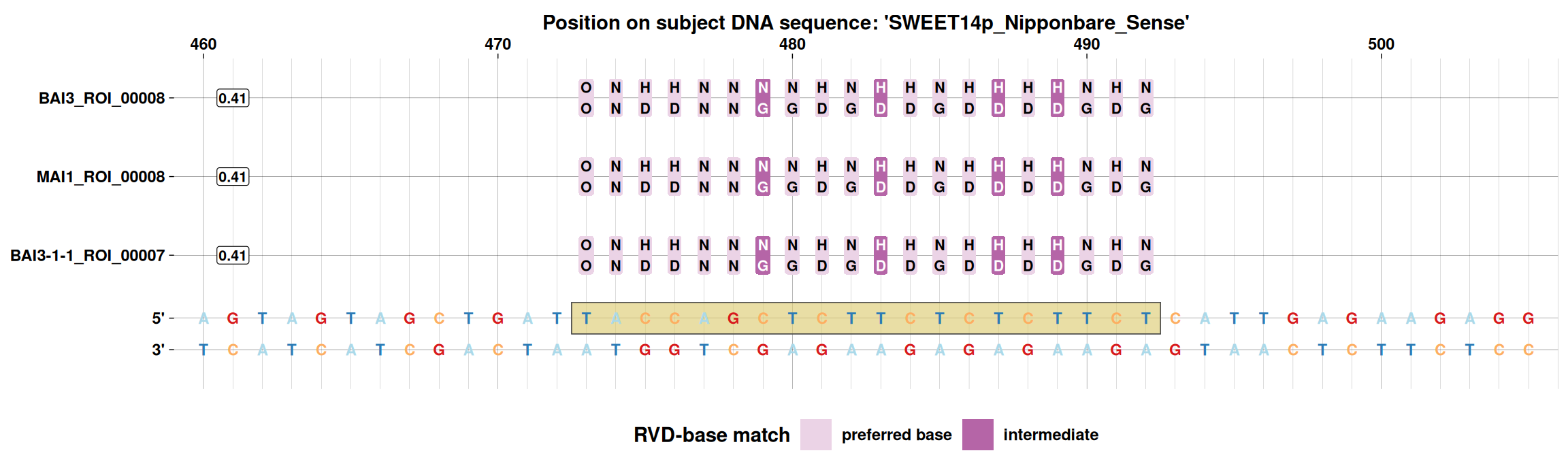
The plot puts each RVD in a box over the base it should contact, and draws the predictions on the sense strand above the sequence and those on the antisense strand below it, since a TALE can bind either strand of its target. The first box, OO, marks position 0: the base just before the first repeat’s target, where TALEs strongly prefer a T. All three predictions in Figure 1 land on the same site with identical scores, as expected of one locus conserved across the three strains.
5 Closing the loop
This set of articles followed one path through a TALE study: tell_tales() to find arrays (correcting them, and checking for what correction could not fix, along the way), tales_compare_distal() and tales_group_hclust()/tales_group_kmedoids() to relate them, tales_align() to see that relatedness directly, and talvez()/preditale() to ask what they do. None of these steps requires the ones before it in code (each function documented here takes ordinary tales objects or plain sequences), but together they cover most of what a study of TALE diversity in a set of genomes actually needs.