The tales_msa class

The tales class article covered tales: one row per part, with dom_code as the identity layer that makes an array alignable. This one is a deep dive into what happens once several arrays are aligned (the tales_msa class) and into the traffic between the two classes: how a tales is promoted into one, how it demotes back, and what each class draws when plotted.

Where this fits

This picks up directly from the alignment built in the walkthrough, with the same three arrays and the same internal gap, and goes further into the mechanics than that article needed to.

Code

library(tantale)
library(dplyr)

1 Building the alignment this article examines

Same three genomes and the same group as the walkthrough, reused here from the cached result of the classification article; see the getting-started article for how these four articles are linked.

tales_align() takes a tales and returns a tales_msa: the same rows, plus one new column, alignment_position. Nothing else changes: every column the input carried, rvd and dom_code both included, survives the trip, because the alignment is computed on one residue layer (residue_col) and the object it returns is still the whole table.

Code

msa <- tales_align(group6, residue_col = "dom_code")
msa
#> <tales_msa> 3 arrays, 18 alignment positions
#>   layers: rvd, dom_code   |   namespace: 5d8762602564ac93   |   8 other columns
#>                       dom_code
#>   MAI1_ROI_00007       84  35  43   5  41  31  24  49  35  54  18  40  31  ...
#>   BAI3_ROI_00007       84  35  43   5  41  31  24  49  35  54  18  40   -  ...
#>   BAI3-1-1_ROI_00006   85  35  43   5  41  31  24  49  35  54  18  40   -  ...

2 What is new: `alignment_position`

A tales_msa is a tales with one extra column and one extra stored number:

alignment_position: where this part sits in the alignment. It agrees with position_in_array up to the first gap and diverges after it.
tales_msa_width(): the alignment’s total column count. It is stored, because max(alignment_position) over a subset of arrays can under-report a width whose last columns happen to be all gaps in that subset.

Code

tales_msa_width(msa)
#> [1] 18

An array on the short side of the internal gap shows the divergence directly: position_in_array counts its 14 real parts contiguously, while alignment_position jumps from 12 to 17 across the gap.

Code

msa |>
  filter(array_id == "BAI3_ROI_00007") |>
  select(array_id, position_in_array, alignment_position, domain_type)
#> # A tibble: 14 × 4
#>    array_id       position_in_array alignment_position domain_type
#>    <chr>                      <int>              <int> <chr>      
#>  1 BAI3_ROI_00007                 1                  1 N-terminus 
#>  2 BAI3_ROI_00007                 2                  2 repeat     
#>  3 BAI3_ROI_00007                 3                  3 repeat     
#>  4 BAI3_ROI_00007                 4                  4 repeat     
#>  5 BAI3_ROI_00007                 5                  5 repeat     
#>  6 BAI3_ROI_00007                 6                  6 repeat     
#>  7 BAI3_ROI_00007                 7                  7 repeat     
#>  8 BAI3_ROI_00007                 8                  8 repeat     
#>  9 BAI3_ROI_00007                 9                  9 repeat     
#> 10 BAI3_ROI_00007                10                 10 repeat     
#> 11 BAI3_ROI_00007                11                 11 repeat     
#> 12 BAI3_ROI_00007                12                 12 repeat     
#> 13 BAI3_ROI_00007                13                 17 repeat     
#> 14 BAI3_ROI_00007                14                 18 C-terminus

Gaps are implicit

There is no row, anywhere, whose alignment_position is a gap: a gap is simply a column with no row for that array. This is why the class validates cheaply and why every tales invariant (the key, the residue columns, the dom_code bijection) keeps holding unchanged on a tales_msa. No rows were added, only a new column that says where each existing row lands.

What the alignment adds on top is its own, narrower set of rules, checked by validate_tales_msa() in addition to everything validate_tales() already checks: alignment_position is a positive integer, present on every row; unique within an array; ordered like position_in_array (an alignment may insert gaps, it may never reorder parts); and never beyond the declared width.

3 Views: matrices are computed on request

The long table is the only thing actually stored. A rectangular alignment (the picture most people have in mind, one row per array, one column per position) is a view, built on request by as.matrix(), which takes the layer to render:

Code

as.matrix(msa, value = "dom_code")
#>                    1    2    3    4   5    6    7    8    9    10   11   12  
#> MAI1_ROI_00007     "84" "35" "43" "5" "41" "31" "24" "49" "35" "54" "18" "40"
#> BAI3_ROI_00007     "84" "35" "43" "5" "41" "31" "24" "49" "35" "54" "18" "40"
#> BAI3-1-1_ROI_00006 "85" "35" "43" "5" "41" "31" "24" "49" "35" "54" "18" "40"
#>                    13   14   15   16   17   18   
#> MAI1_ROI_00007     "31" "24" "49" "45" "29" "100"
#> BAI3_ROI_00007     NA   NA   NA   NA   "29" "100"
#> BAI3-1-1_ROI_00006 NA   NA   NA   NA   "29" "100"

Code

as.matrix(msa, value = "rvd")
#>                    1       2    3    4    5    6    7    8    9    10   11  
#> MAI1_ROI_00007     "NTERM" "NN" "HD" "NV" "HD" "NI" "NG" "NI" "NN" "NS" "HD"
#> BAI3_ROI_00007     "NTERM" "NN" "HD" "NV" "HD" "NI" "NG" "NI" "NN" "NS" "HD"
#> BAI3-1-1_ROI_00006 "NTERM" "NN" "HD" "NV" "HD" "NI" "NG" "NI" "NN" "NS" "HD"
#>                    12   13   14   15   16   17   18     
#> MAI1_ROI_00007     "HD" "NI" "NG" "NI" "NG" "NI" "CTERM"
#> BAI3_ROI_00007     "HD" NA   NA   NA   NA   "NI" "CTERM"
#> BAI3-1-1_ROI_00006 "HD" NA   NA   NA   NA   "NI" "CTERM"

Both matrices have the same shape and the same gaps, because both read the same alignment. This is what lets plot.tales_msa() (below) show a domain’s identity as a colour and its RVD as a label on the same cell, termini included, since termini carry an RVD-string entry (their NTERM/CTERM marker) just as repeats do.

4 Coercion between `tales` and `tales_msa`

Promotion is tales_align(): give it a complete tales, get back a tales_msa. There is no other route, because the alignment column has to come from an actual alignment run.

Demotion is as_tales():

Code

demoted <- as_tales(msa)
class(demoted)
#> [1] "tales"      "tbl_df"     "tbl"        "data.frame"

Code

is_tales_msa(demoted)
#> [1] FALSE
"alignment_position" %in% names(demoted)
#> [1] TRUE

alignment_position survives as an ordinary column, so demoting keeps where things were aligned. What goes is the object’s claim to be a single coherent alignment, and the stored width goes with it:

Code

tales_msa_width(demoted)
#> NULL

Why the distinction matters

A talome-wide summary spanning several independently aligned groups cannot be one tales_msa: each group has its own width and its own coordinate system, so alignment_position = 5 would mean unrelated things in two different groups. The right shape for that case is a plain tales carrying alignment_position as an ordinary column, meaningful within each group.

Subsetting degrades the same way, automatically, one step at a time. Row subsetting never touches the alignment contract, since every check above still holds on a subset of rows. Column subsetting can: dropping alignment_position itself leaves something that is still a valid tales (everything else about a part is unaffected) but can no longer be a tales_msa, and the class notices without being told:

Code

no_alignment <- msa |> select(-alignment_position)
class(no_alignment)
#> [1] "tales"      "tbl_df"     "tbl"        "data.frame"

This is the same graded-degradation mechanism from the tales class article’s [.tales method, one level up: a tales_msa that loses what makes it an alignment steps down to a tales, and a tales that loses its key steps down to a bare tibble, for the same reason. Losing an optional column (seqnames, aa_seq) costs nothing at either level.

5 Plotting: two methods, one generic

plot() dispatches on class, so the two objects draw different things from the same call.

5.1 `plot.tales()` before and after alignment

A tales without an alignment can only be laid out on position_in_array: every array starts its own count at 1, so a feature shared by all arrays sits wherever it happens to fall in each. position = "alignment" needs the column that only an aligned (or demoted-from-aligned) object carries, and lines features up instead. The final half-repeat shows it: at position 13 in BAI3 and BAI3-1-1 and 17 in MAI1 before alignment, in column 17 for all three after.

Code

plot(group6, position = "array")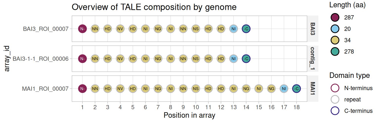

Figure 1: The same three arrays laid out by position_in_array: no gaps, because nothing has been aligned.

Code

plot(demoted, position = "alignment")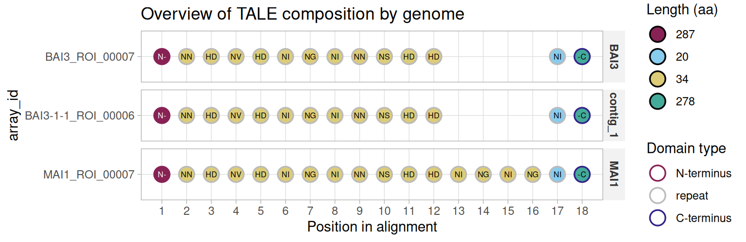

Figure 2: The same three arrays laid out by alignment_position: the four-repeat gap now shows as columns 13-16.

5.2 `plot.tales_msa()`: three things decided independently

The alignment plot draws a heatmap (one row per array, one column per position) and three questions about it are answered separately:

what each cell says: label, defaulting to rvd whenever that is not also the fill layer;
what colour that text is: always whether the cell matches the consensus of its column (tales_consensus()), black for yes, red for no, grey where the consensus is a gap, regardless of what fill_type is showing;
what colour the block behind it is: fill_type, the only one of the three that can be unavailable.

fill_type	shows	needs
`"domain_clust"`	which cluster the domain falls in, cut at `h_cut`	`domain_distances`
`"domain_sim"`	protein-sequence similarity to the reference, 0-100	`domain_distances`
`"rvd_sim"`	how alike the RVD’s DNA-binding preference is to the reference’s, -1 to 1	a `label` layer

The domain_distances argument takes exactly that: the domain_distances element of tales_compare_distal()’s result. Passing tale_distances (the tale_distances element) in addition adds a dendrogram panel ordering the rows by relatedness:

Code

plot(msa, tale_distances = cmp$tale_distances, domain_distances = cmp$domain_distances)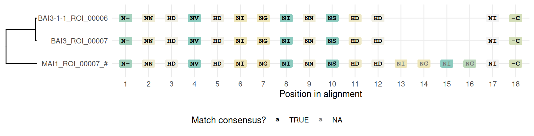

Figure 3: Default plot.tales_msa() view: domain-cluster fill, RVD labels, and a tree from tale_distances.

"rvd_sim" asks a different question at a different layer: how alike each RVD’s DNA-binding specificity is to the reference’s. It needs no domain_distances at all, only the RVDs themselves:

Code

plot(msa, fill_type = "rvd_sim")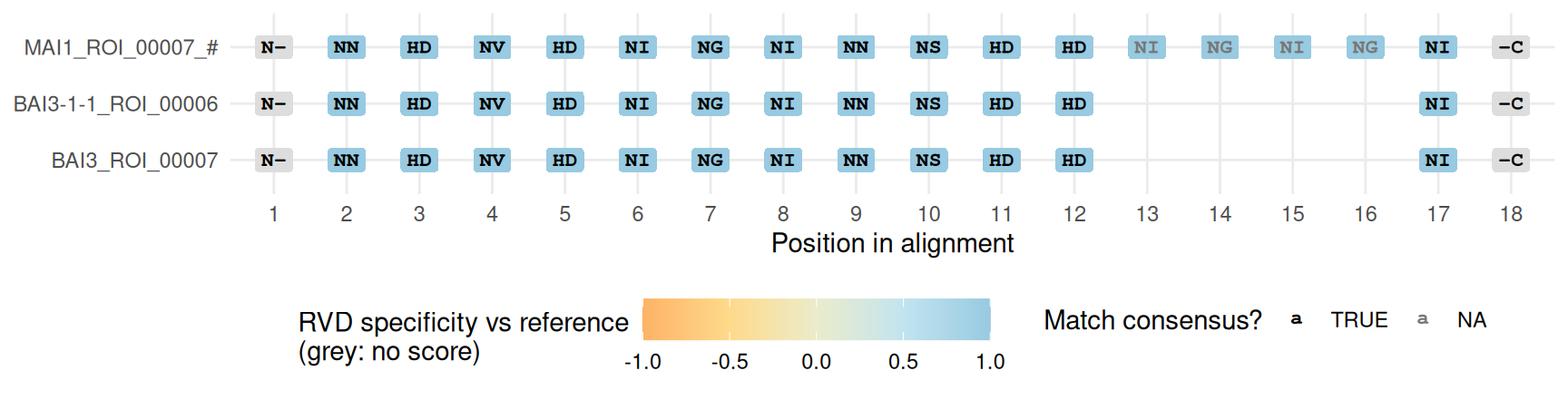

Figure 4: The same alignment, coloured by RVD specificity relative to the reference.

Here every repeat carries the same RVD as the reference’s at its position, so all score 1. That includes NV, which the built-in similarity table (TALVEZ’s, 17 RVDs) does not cover: an RVD identical to the reference’s always scores 1. Termini have no DNA-binding preference and stay grey.

The domain- and RVD-level views genuinely differ: repeats carrying HD and ND differ in sequence yet both favour cytosine, while repeats differing only at positions 12-13 are near-identical proteins that target different bases. "domain_sim" and "rvd_sim" answer two different questions.

6 Next

Return to the walkthrough to continue with target prediction, or to the tales class article for the identity layer this alignment is built on.

1 Building the alignment this article examines

2 What is new: alignment_position

3 Views: matrices are computed on request

4 Coercion between tales and tales_msa

5 Plotting: two methods, one generic

5.1 plot.tales() before and after alignment

5.2 plot.tales_msa(): three things decided independently

6 Next

2 What is new: `alignment_position`

4 Coercion between `tales` and `tales_msa`

5.1 `plot.tales()` before and after alignment

5.2 `plot.tales_msa()`: three things decided independently